library(Seurat)
library(SeuratWrappers)
library(monocle3)
library(UCell)
library(dbscan)
library(ggplot2)
library(dplyr)

# Loading the CytoTRACE code.
source(here::here("./data/CytoTRACE.R"))
source(here::here("./data/plotCytoTRACE.R"))The rooting problem for pseudotime analysis
There are many reasons why a researcher wants to perform pseudotime analysis on single-cell datasets, including but not limited to cellular differentiation, developmental stages, and disease progression.
Currently, we can leverage many packages for dealing with such analysis. We could roughly categorize them into approaches based on user-defined roots and model-based roots. Note that roots are the starting point of the pseudotime analysis, i.e., the algorithm will sort the cells and their transcriptional profiles based on that specific data point. Therefore, it is a VERY crucial step in pseudotime!
On that note, Monocle3 is a well-known package for performing pseudotime analysis. It should be included in the “user-defined” category, i.e., it relies on a knowledge-driven selection. To aid bioinformaticians in root selection, we can leverage distinct models to give us hints. Today, we will talk about CytoTRACE, a package for measuring differentiation scores in single-cell datasets. CytoTRACE is based on the simple observation that transcriptional diversity—the number of genes expressed in a cell—decreases during differentiation. Thus, we can assume that cells predicted as less differentiated are the best candidates for pseudotime roots. Check it out!
1. Loading requirements
2. Loading pre-processed Seurat object
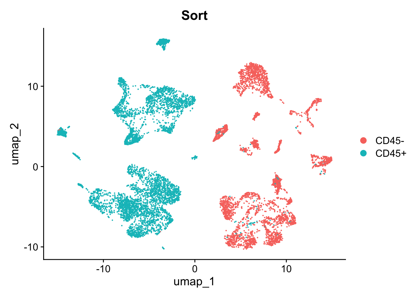
Here, we will leverage data from Vázquez-García et al (2022). This data was subset for only 20.000 cells, including malignant and TME cells. Particularly, this dataset was CD45+ and CD45− flow-sorted, i.e., we can easily distinguish between putative malignant, epithelial cells and TME-related cells.
seurat_object <- readRDS(file = here::here("./data/Ovarian_main_cluster_object.20k.RDS"))3. Performing basic cell-type annotation
Next, we will subset NK cells based on lineage markers. It is fairly easy to do once we know which genes to look at. We will provide a small, but accurate list for major cell types.
cell_lineage_markers <- list(
  "T-Cells" = c("CD3D","CD3E","CD4","CD8A","CD8B"),
  "NK_cells" = c("NCAM1","KLRG1","FCGR3A","NKG7","GNLY","CD160"),
  "B/Plasma_cells" = c("CD19","MS4A1","CD79A","CD79B","SDC1","MZB1","XBP1","JCHAIN"),
  "Myeloid" = c("LYZ","S100A8","S100A9","CD68","CD14","C1QB","C1QC"),
  "Endothelial" = c("PECAM1","VWF","ENG","MCAM"),
  "Fibroblast" = c("FAP","PDPN","COL1A2","DCN","COL3A1","COL6A1"),
  "Epithelial" = c("EPCAM","MUC1","ERBB2","KRT8","PGC","GKN2","SLC5A5","FABP1","KRT20")
)
seurat_object <- AddModuleScore_UCell(
seurat_object,
ncores = 8,
features = cell_lineage_markers) 4. Subsetting NK compartment for CytoTRACE analysis
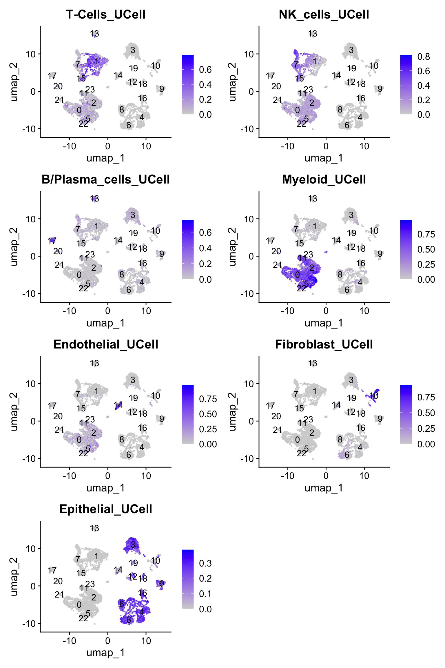
As expected the signature score derived from UCell can help us to annotate the distinct cell populations. The clusters #1, #7, and #15 are associated with NK and T-cells. This tutorial will consider that clusters #7 and #15 are populated by NK cells. Note, that cluster #15 displays both T and NK signatures, a common feature associated with NK/T-cells. However, we will ignore it for today :)
nk_compartiment_object <- subset(
  seurat_object, subset = seurat_clusters %in% c(7, 15))
nk_compartiment_counts <- LayerData(
object = nk_compartiment_object, layer = "counts")cyto_results <- CytoTRACE(nk_compartiment_counts)5. Extracting less differentiated NK cells
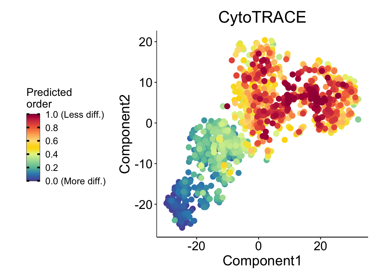
CytoTRACE will rank the cell based on differentiation score, values ranging from 0 (more differentiated) to 1 (less differentiated).
# Extracting UMAP coordinates
nk_compartiment_embeddings <- Embeddings(
  nk_compartiment_object[["umap"]]
)

# Adding UMAP and CytoTRACE score on metadata
nk_compartiment_object <- AddMetaData(
  nk_compartiment_object,
  nk_compartiment_embeddings
)

nk_compartiment_object@meta.data[['CytoTRACE']] <-
  cyto_results$CytoTRACE
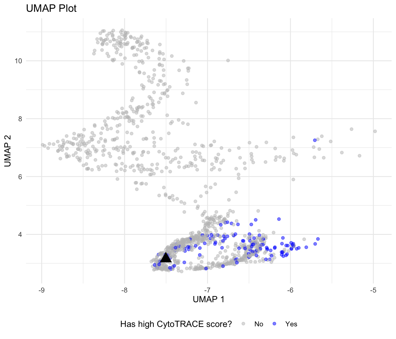
Next, we will leverage dbscan for selecting highly-dense clusters with CyTRACE scores higher or equal to 0.9.
# Creating a data.frame with embeddings and CytoTrace score
data <- nk_compartiment_object@meta.data[, c("umap_1", "umap_2", "CytoTRACE")]
data <- data %>%
  mutate(
    filtered = ifelse(CytoTRACE >= 0.9, "Yes", "No")
  )
# Subsetting only CytoTRACE higher than 0.9 (less differentiated)
filtered_data <- data %>%
filter(filtered == "Yes") %>%
select(umap_1, umap_2)
# Choose eps and minPts based on your dataset characteristics
clustering <- dbscan(filtered_data, eps = 0.5, minPts = 5)# Calculate k-nearest neighbors distance as a proxy for density
distances <- kNNdist(filtered_data, k = 5) # You might want to adjust this based on the density you expect
# Add distances to your data frame
filtered_data$local_density = 1 / distances # Inverse of distance to indicate density
# Determine the candidate/representative for each cluster
cluster_representatives <- data.frame()
for (i in unique(clustering$cluster)) {
if (i > 0) {
# Only consider non-noise clusters
cluster_data <- filtered_data[clustering$cluster == i,]
# Select the data point with the maximum local density
representative_index <- which.max(cluster_data$local_density)
cluster_representatives <- rbind(cluster_representatives, cluster_data[representative_index, ])
}
}
knitr::kable(cluster_representatives)| umap_1 | umap_2 | local_density | |
|---|---|---|---|
| SPECTRUM-OV-009_S1_CD45P_RIGHT_UPPER_QUADRANT_AATCGACAGACGGTTG-1 | -7.502961 | 3.156997 | 15.18489 |
ggplot(data = data, aes(x = umap_1, y = umap_2)) +
  geom_point(aes(color = filtered), alpha = 0.5) +
  geom_point(data = cluster_representatives, color = "black", size = 5, shape = 17) +
  scale_color_manual(values = c("grey", "blue", "black"), labels = c("No", "Yes", "Candidate")) +
  labs(title = "UMAP Plot", x = "UMAP 1", y ="UMAP 2", color = "Has high CytoTRACE score?") +
  theme_minimal() +
  theme(legend.position = "bottom")
Okey dokey! Now we have a decent candidate (black triangle) to be used as a root! We can finally focus on pseudotime analysis with Monocle3.
6. Preparing Monocle object
monocle_object <- as.cell_data_set(nk_compartiment_object)
monocle_object <- cluster_cells(monocle_object)
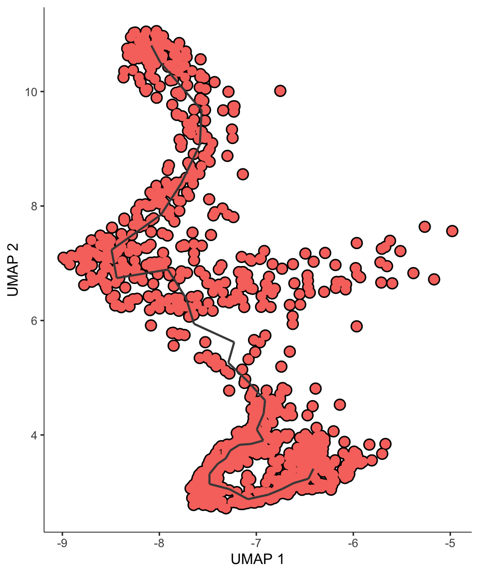
monocle_object <- learn_graph(monocle_object)7. Defining pseudotime root based on differentiation score
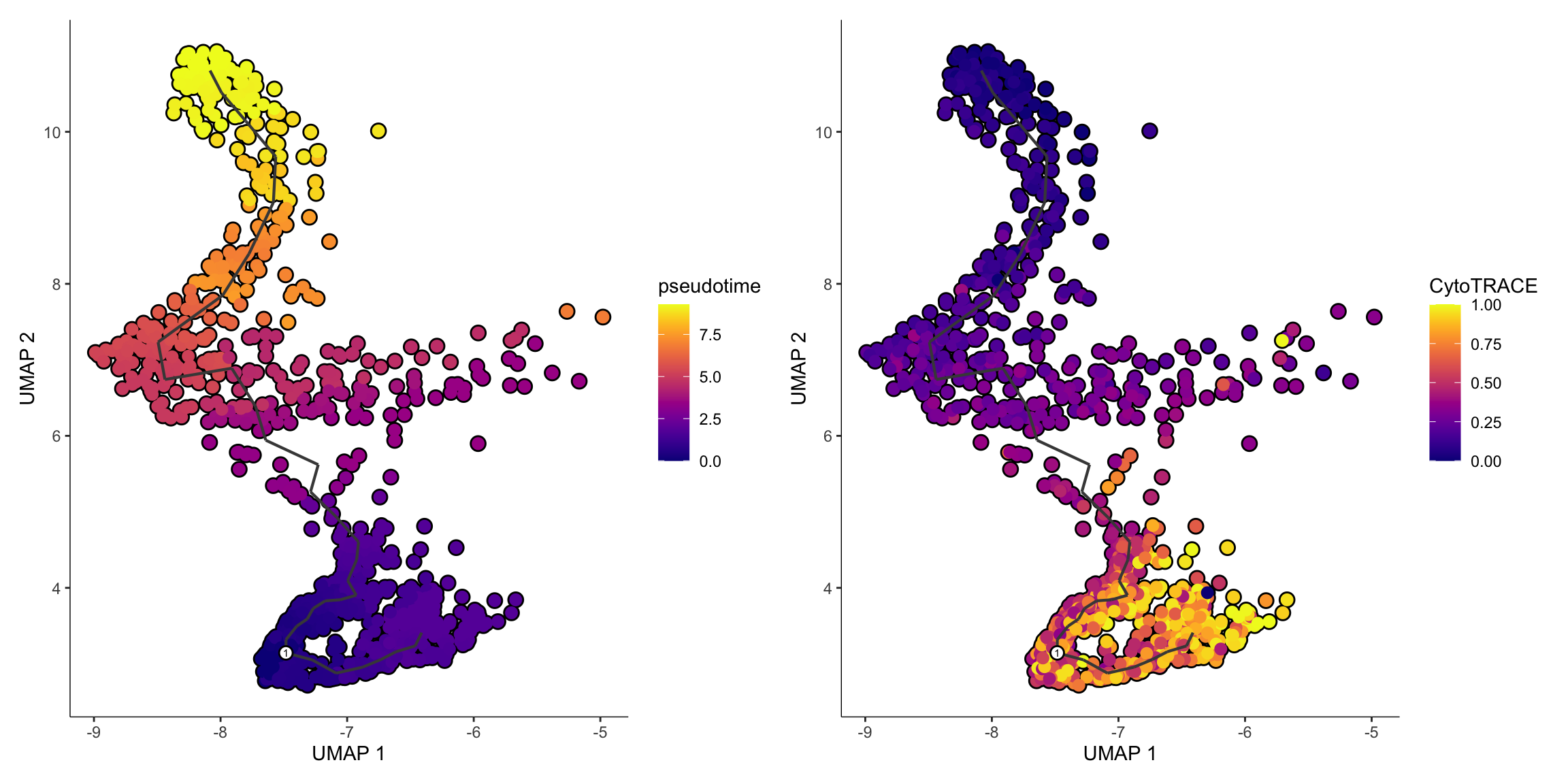
monocle_object <- order_cells(
  monocle_object, root_cells = row.names(cluster_representatives)) # Voilà. We can add the cell_id here.
p1 <- plot_cells(
monocle_object,
color_cells_by = "pseudotime",
cell_size = 2,
label_cell_groups = FALSE,
label_leaves = FALSE,
label_branch_points = FALSE
)
p2 <- plot_cells(
monocle_object,
color_cells_by = "CytoTRACE",
cell_size = 2,
label_cell_groups = FALSE,
label_leaves = FALSE,
label_branch_points = FALSE
)
p1 + p2Done! We now have a basic workflow for defining pseudotime roots without manual intervention. The CytoTRACE + Monocle3 idea was originally published here.
R version 4.3.0 (2023-04-21)
Platform: aarch64-apple-darwin22.4.0 (64-bit)
Running under: macOS Ventura 13.6.6

Matrix products: default
BLAS:   /opt/local/Library/Frameworks/R.framework/Versions/4.3/Resources/lib/libRblas.dylib
LAPACK: /opt/local/Library/Frameworks/R.framework/Versions/4.3/Resources/lib/libRlapack.dylib;  LAPACK version 3.11.0

locale:
[1] en_US.UTF-8/en_US.UTF-8/en_US.UTF-8/C/en_US.UTF-8/en_US.UTF-8

time zone: America/Chicago
tzcode source: internal

attached base packages:
[1] stats4    stats     graphics  grDevices utils     datasets  methods
[8] base

other attached packages:
 [1] dplyr_1.1.2                 ggplot2_3.4.2
 [3] dbscan_1.1-11               UCell_2.6.2
 [5] monocle3_1.3.4              SingleCellExperiment_1.23.0
 [7] SummarizedExperiment_1.31.1 GenomicRanges_1.53.1
 [9] GenomeInfoDb_1.37.2         IRanges_2.35.2
[11] S4Vectors_0.39.1            MatrixGenerics_1.13.1
[13] matrixStats_1.0.0           Biobase_2.61.0
[15] BiocGenerics_0.47.0         SeuratWrappers_0.3.19
[17] Seurat_4.9.9.9045           SeuratObject_4.9.9.9084
[19] sp_2.0-0

loaded via a namespace (and not attached):
  [1] RcppAnnoy_0.0.21        splines_4.3.0           later_1.3.1
  [4] bitops_1.0-7            tibble_3.2.1            R.oo_1.25.0
  [7] polyclip_1.10-4         fastDummies_1.7.3       lifecycle_1.0.3
 [10] rstatix_0.7.2           rprojroot_2.0.3         globals_0.16.2
 [13] lattice_0.21-8          MASS_7.3-60             backports_1.4.1
 [16] magrittr_2.0.3          plotly_4.10.2           rmarkdown_2.23
 [19] yaml_2.3.7              remotes_2.4.2.1         httpuv_1.6.11
 [22] sctransform_0.3.5       spam_2.9-1              spatstat.sparse_3.0-2
 [25] reticulate_1.35.0       cowplot_1.1.1           pbapply_1.7-2
 [28] minqa_1.2.5             RColorBrewer_1.1-3      abind_1.4-5
 [31] zlibbioc_1.47.0         Rtsne_0.16              purrr_1.0.2
 [34] R.utils_2.12.2          RCurl_1.98-1.12         GenomeInfoDbData_1.2.10
 [37] ggrepel_0.9.3           irlba_2.3.5.1           listenv_0.9.0
 [40] spatstat.utils_3.0-3    terra_1.7-39            goftest_1.2-3
 [43] RSpectra_0.16-1         spatstat.random_3.1-5   fitdistrplus_1.1-11
 [46] parallelly_1.36.0       ncdf4_1.21              leiden_0.4.3
 [49] codetools_0.2-19        DelayedArray_0.27.10    tidyselect_1.2.0
 [52] farver_2.1.1            viridis_0.6.4           lme4_1.1-34
 [55] spatstat.explore_3.2-1  jsonlite_1.8.7          BiocNeighbors_1.19.0
 [58] ellipsis_0.3.2          progressr_0.13.0        ggridges_0.5.4
 [61] survival_3.5-5          tools_4.3.0             ica_1.0-3
 [64] Rcpp_1.0.11             glue_1.6.2              gridExtra_2.3
 [67] SparseArray_1.1.11      xfun_0.39               here_1.0.1
 [70] withr_2.5.0             BiocManager_1.30.21.1   fastmap_1.1.1
 [73] HiClimR_2.2.1           boot_1.3-28.1           fansi_1.0.4
 [76] egg_0.4.5               digest_0.6.33           rsvd_1.0.5
 [79] R6_2.5.1                mime_0.12               colorspace_2.1-0
 [82] scattermore_1.2         tensor_1.5              spatstat.data_3.0-1
 [85] R.methodsS3_1.8.2       utf8_1.2.3              tidyr_1.3.0
 [88] generics_0.1.3          data.table_1.14.8       robustbase_0.99-0
 [91] httr_1.4.6              htmlwidgets_1.6.2       S4Arrays_1.1.5
 [94] uwot_0.1.16             pkgconfig_2.0.3         gtable_0.3.3
 [97] lmtest_0.9-40           XVector_0.41.1          pcaPP_2.0-3
[100] htmltools_0.5.5         carData_3.0-5           dotCall64_1.0-2
[103] scales_1.2.1            png_0.1-8               knitr_1.43
[106] rstudioapi_0.15.0       reshape2_1.4.4          nlme_3.1-162
[109] nloptr_2.0.3            proxy_0.4-27            zoo_1.8-12
[112] stringr_1.5.0           KernSmooth_2.23-22      parallel_4.3.0
[115] miniUI_0.1.1.1          pillar_1.9.0            grid_4.3.0
[118] vctrs_0.6.3             RANN_2.6.1              ggpubr_0.6.0
[121] promises_1.2.0.1        car_3.1-2               xtable_1.8-4
[124] cluster_2.1.4           evaluate_0.21           mvtnorm_1.2-2
[127] cli_3.6.1               compiler_4.3.0          rlang_1.1.1
[130] crayon_1.5.2            leidenbase_0.1.25       ggsignif_0.6.4
[133] future.apply_1.11.0     labeling_0.4.2          plyr_1.8.8
[136] stringi_1.7.12          nnls_1.5                viridisLite_0.4.2
[139] deldir_1.0-9            BiocParallel_1.35.3     assertthat_0.2.1
[142] ccaPP_0.3.3             munsell_0.5.0           lazyeval_0.2.2
[145] spatstat.geom_3.2-4     Matrix_1.6-0            RcppHNSW_0.4.1
[148] patchwork_1.1.2         future_1.33.0           shiny_1.7.4.1
[151] ROCR_1.0-11             broom_1.0.5             igraph_1.5.1
[154] DEoptimR_1.1-0 