Lexanomics Blog - Yet another tip for speeding up DEG analysis on Seurat

Not long ago, we discussed ways to speed up differential expression analysis in single-cell datasets.

For that, I wrote a quick snippet using the future package for parallelizing. This is 100% cool. But, recently I found a more convenient way to do such a task. On this note, since an old dog can still learn new tricks, I would like to introduce: presto.

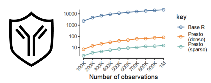
Presto is a Wilcoxon rank sum test and auROC implementation that can run 1 million observations, 1K features, and 10 groups in 16 seconds (sparse input) and 85 seconds (dense input) 1. Yes, sir, we are fast.

However, presto isn’t a very new tool! It has been around for at least 5 years (based on GitHub development). Yet, it became much more convenient once it was integrated into the Seurat package (version 5.1.0) 2.

Let’s do a quick and dirty hands-on.

First, we need to load the package and the data we will use for this example. I will use the same data that I used in this debugging new post.

1. Loading requirements

library(Seurat)
library(dplyr)
library(presto) # Optional. It will be loaded behind the scenes.

2. Loading pre-processed Seurat object

seurat_object <- readRDS(file = here::here("./data/Ovarian_main_cluster_object.20k.RDS"))

3. Running DEG analysis across clusters

start_time <- Sys.time()

# Find markers for every cluster compared to all remaining cells, report only the positive
seurat_markers <- FindAllMarkers(seurat_object, only.pos = TRUE)

end_time <- Sys.time()

What?! How is that? I haven’t change my code at all.

Yes, young bioinformatician. I said it was convenient everything you need for running it is already in place in Seurat version 5.1.0. For those not using this versions, you can also rely on SeuratWrappers. This package has a function called RunPrestoAll.

4. Inspecting DEG table

seurat_markers %>%
  group_by(cluster) %>%
  select(cluster, gene, pct.1, pct.2, avg_log2FC, p_val) %>%
  top_n(5)

# A tibble: 110 × 6
# Groups:   cluster [22]
   cluster gene            pct.1 pct.2 avg_log2FC   p_val
   <fct>   <chr>           <dbl> <dbl>      <dbl>   <dbl>
 1 0       SLC26A1         0.01  0.004      0.798 0.00631
 2 0       NATD1           0.037 0.024      0.246 0.00740
 3 0       SLC35G1         0.012 0.005      0.428 0.00770
 4 0       ENSG00000273088 0.022 0.012      0.145 0.00832
 5 0       CTSK            0.041 0.027      0.903 0.00873
 6 1       TMSB15B.1       0.012 0.006      2.82  0.00975
 7 1       PGLYRP2         0.018 0.01       1.93  0.00975
 8 1       ZNF585B         0.016 0.031      0.418 0.00977
 9 1       ZNF567          0.078 0.111      0.785 0.00983
10 1       SOBP            0.011 0.023      0.128 0.00988
# ℹ 100 more rows

Pretty cool, right? Identical results, but much faster.

5. Measuring computational time

computational_time <- round(end_time - start_time, 2)

Tip

Yeah, we ran the FindAllMarkers function into 39.65 seconds. The authors claimed that it could be 295 times faster than conventional implementations. Do not trust them? Feel free to run it. Hint: You might need to change your Seurat version. Also, you can use the toy dataset in this tutorial, it can be found here.

References

Korsunsky, Ilya, Aparna Nathan, Nghia Millard, and Soumya Raychaudhuri. 2019. “Presto Scales Wilcoxon and auROC Analyses to Millions of Observations.” bioRxiv. https://doi.org/10.1101/653253.